Stefan's family rented a rototiller to prepare an area in their backyard for spring planting. The rental company charged an init

Answer: Circle C has a radius of 7 cm.

Explanation:

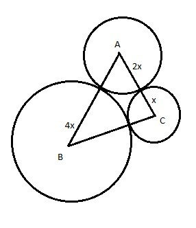
Referring to the illustration below:

Let's denote the radius of circle C as x.

Circle A's radius can be represented as 2x.

Circle B's radius can be expressed as 4x.

The length of side AC in triangle ΔABC becomes x + 2x = 3x.

For side BC of triangle ΔABC, we get 4x + x = 5x.

Similarly, for side AB of triangle ΔABC, it is 4x + 2x = 6x.

Given that the perimeter of triangle ΔABC totals 98 cm.

Remember, the perimeter refers to the total length around the triangle.

Hence, Perimeter = 6x + 5x + 3x = 98 cm.

Thus, 14x = 98.

From this, we find x = .

Therefore, x = 7.

This concludes that the radius of circle C is 7 cm.

Kayla's opportunity cost for attending the movie is $9.50

Tara's total expense for watching the movie amounts to $50.50

Answer:

in steps

Step-by-step explanation:

In a fair roulette game, the likelihood of the ball landing on RED remains constant, regardless of prior spins.

a) 18/38

b) 18/38

c) Yes, I have confidence in my responses. Since it's fair, the number of RED slots does not change.

Response:

Detailed explanation:

Hello!

Stratified sampling involves the categorization of the population into subgroups based on pre-established criteria for the study. These subgroups consist of homogeneous units concerning the relevant characteristics. In this instance, individuals in the groups will represent only one of the two potential opinions (support or not support) and not both.

The researcher determines the sample size desired, considering several factors such as finances, material availability, and accessibility to experimental subjects (for instance, if they are endangered species, larger sample sizes may not be feasible).

One might conduct proportionate stratified sampling by selecting a proportion of respondents who answered "yes" along with those who answered "no."

In this sampling method, taking a specific proportion from each subgroup allows for a more straightforward extrapolation of results to the overall populations. For example, if you needed a sample size of n = 20, each stratum would ideally contain half, meaning 10 from the “yes” group and 10 from the “no” group.

I hope this is helpful!

A. The order in which you define the variables isn't fixed. For the sake of this discussion, let's define them like this:

x = Number of bookshelves
y = Number of tables

B. Due to the total number of items to produce, we have the following inequality based on those variables.

x + y > 25

Additionally, you can create a second inequality concerning your budget for materials.

20x + 45y < 675

Moreover, you should also add that both values must not be negative, since you can't produce negative tables.

C. By analyzing the constraints and solving the system, you will find that the feasible region contains 4 vertices.

(0,0)
(18, 7)
(0, 15)
(33.75, 0) or (33, 0) if you prefer to round it.