Y = 5x + 3
y = 5.5x + 2
0.5x = 1
x = 2
y = 13
I trust this information will assist you. c:
Answer:
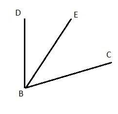
m∠EBC=34°
Step-by-step explanation:
We establish that
m∠DBC=m∠DBE+m∠EBC
Refer to the accompanying diagram for clarity on the issue
Replace the known values in the equation and determine x

Calculate the size of angle EBC
m∠EBC=(3x+13)°
Insert the value for x
m∠EBC=(3(7)+13)°
m∠EBC=(21+13)°
m∠EBC=34°
Hi! The goal of the Chi-Square Goodness of Fit test is to determine if observed frequencies of a categorical variable align with the expected historical or theoretical values in the population. Having the sales proportions of the top-five compact cars, we compare them against 400 compact car sales data from Chicago to see if there are discrepancies. Specifically, we have:
- Chevy Cruze 24% ⟹ P(CC) = 0.24
- Ford Focus 21% ⟹ P(FF) = 0.21
- Hyundai Elantra 20% ⟹ P(HE) = 0.20
- Honda Civic 18% ⟹ P(HC) = 0.18
- Toyota Corolla 17% ⟹ P(TC) = 0.17
The hypotheses established are:
H₀: P(CC) = 0.24; P(FF) = 0.21; P(HE) = 0.20; P(HC) = 0.18; P(TC) = 0.17
H₁: There is a discrepancy between expected and observed outcomes.
With α set at 0.05, the statistic calculated is based on Oi (observed frequency) and Ei (expected frequency). The initial step involves calculating expected frequencies using: Ei = n * Pi, where Pi is the theoretical proportion for each category stated in the null hypothesis. The test conducted is right-tailed, and so is the p-value, calculated as: P(X²₄ ≥ 11.23) = 1 - P(X²₄ < 11.23) = 1 - 0.98 = 0.02. Since the p-value is lower than α, we reject the null hypothesis, indicating that Chicago's market shares for the five compact cars differ from those reported by Motor Trend.
Answer: See explanation
Step-by-step explanation:
To determine how many boxes of sugar Alonso can purchase, we can express the scenario as follows:
= 2.75 + 11.50S ≤ 55
Expanding this gives us:
2.75 + 11.50S ≤ 55
11.50S ≤ 55 - 2.75
11.50S ≤ 52.25
S ≤ 52.25 / 11.50
S ≤ 4.54
Thus, he is able to buy 4 boxes of sugar.