Answer:
The average for the sampling distribution of the sample proportion is 0.29
The standard deviation for this sampling distribution is 0.01435
Step-by-step explanation:
The mean of the sampling distribution for the sample proportion equals the actual population proportion, which is p = 0.29 in this scenario.
The standard deviation for the sampling distribution of the sample proportion is computed as follows;

Utilizing the provided values;
p = 0.29
1 - p = 0.71
n = 1000
The standard deviation computes to;

Thus, the standard deviation is 0.01435.
$200 was the original amount before any discounts, and he paid $136.
Response:
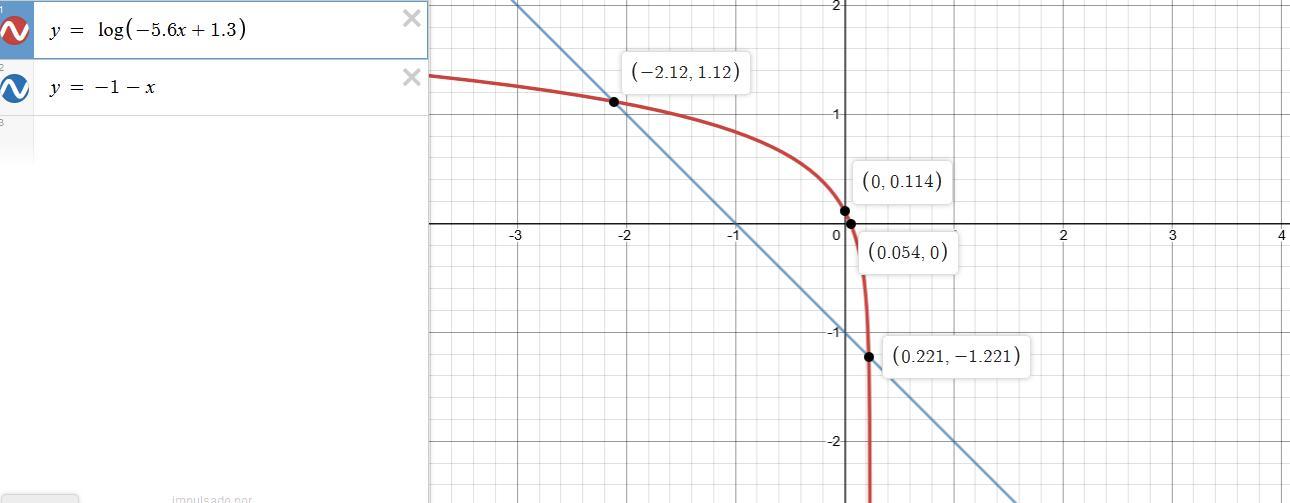
- Refer to the attached graph
Clarification:
To analyze log (−5.6x + 1.3) = −1 − x visually, graph these equations on the same coordinate system:
- Equation 1: y = log (5.6x + 1.3)
The first equation can be graphed using these characteristics of logarithmic functions:
- Domain: values must be positive ⇒ -5.6x + 1.3 > 0 ⇒ x < 13/56 (≈ 0.23)
- Range: all real values (- ∞, ∞)
log ( -5.6x + 1.3) = 0 ⇒ -5.6x + 1.3 = 1 ⇒ x = 0.3/5.6 ≈ 0.054
x = 0 ⇒ log (0 + 1.3) = log (1.3) ≈ 0.11
- Choose additional values to create a table:
x log (-5.6x + 1.3)
-1 0.8
-2 1.1
-3 1.3
- This graph is shown in the attached image: it's represented by the red curve.
Graphing the second equation is simpler as it forms a straight line: y = - 1 - x
- slope, m = - 1 (the coefficient of x)
- y-intercept, b = - 1 (the constant term)
- x-intercept: y = 0 = - 1 - x ⇒ x = - 1
- This graph is indicated by the blue line in the image.
The resolution to the equations corresponds to the points where the two graphs intersect. The graphing method thus allows you to determine the x coordinates of these intersection points. Ordered from smallest to largest, rounded to the nearest tenth, we have: